Basic linear algebra notes
by Rishi Jain
I wanted to go back and pin down the basics of linear algebra properly, since so much of what I want to learn next leans on them, so these are my notes from working back through the foundations, cleaned up enough to share. They follow Zachary Huang’s Give Me 30 min, I will make Linear Algebra Click Forever, roughly one section per idea, with the small numerical examples worked out and a short NumPy snippet for each. There is nothing past the foundations here, and they might be useful if you are making the same pass.
Vectors and the dot product
Start with three vectors,
\[ a = [5,\, 4,\, 1], \qquad b = [4,\, 5,\, 2], \qquad c = [1,\, 2,\, 5] \]
and drawn from the origin, they live in 3D space:
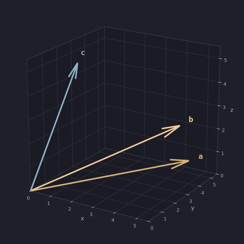
Here \( a \) and \( b \) (gold) sit close together, while \( c \) (blue) heads off on its own. The smaller the angle between two vectors, the more similar they are, and the dot product is what turns that similarity into a single number. It has two formulas that describe the same quantity.
The first is the calculation formula, which multiplies matching components and adds them up,
\[ a \cdot b = a_1 b_1 + a_2 b_2 + a_3 b_3 + \dots + a_n b_n \]
and the second is the geometric formula, which connects the dot product to the angle \( \theta \) between the vectors,
\[ a \cdot b = \lVert a \rVert \, \lVert b \rVert \cos\theta \]
where the length, or norm, of a vector is
\[ \lVert a \rVert = \sqrt{a_1^2 + a_2^2 + \dots + a_n^2} \]
To recover the angle we run both formulas against each other. We get \( a \cdot b \) from the calculation formula, compute the two lengths \( \lVert a \rVert \) and \( \lVert b \rVert \), and then rearrange the geometric formula for \( \theta \),
\[ \cos\theta = \frac{a \cdot b}{\lVert a \rVert \, \lVert b \rVert} \]
Worked out for \( a \) and \( b \):
\[ a \cdot b = (5)(4) + (4)(5) + (1)(2) = 20 + 20 + 2 = 42 \]
\[ \lVert a \rVert = \sqrt{5^2 + 4^2 + 1^2} = \sqrt{42} \approx 6.48 \]
\[ \lVert b \rVert = \sqrt{4^2 + 5^2 + 2^2} = \sqrt{45} \approx 6.71 \]
\[ \cos\theta = \frac{42}{6.48 \times 6.71} \approx 0.966 \qquad\Rightarrow\qquad \theta = \arccos(0.966) \approx 15.0^\circ \]
Not much of an angle. \( a \) and \( b \) are similar, so \( \theta \) comes out small. Now \( a \) and \( c \), which look rather less alike:
\[ a \cdot c = (5)(1) + (4)(2) + (1)(5) = 5 + 8 + 5 = 18 \]
\[ \lVert a \rVert \approx 6.48, \qquad \lVert c \rVert = \sqrt{30} \approx 5.48 \]
\[ \cos\theta = \frac{18}{6.48 \times 5.48} \approx 0.507 \qquad\Rightarrow\qquad \theta = \arccos(0.507) \approx 59.5^\circ \]
This is cosine similarity: similar vectors give a cosine near 1 and a small angle, and dissimilar ones give a smaller cosine and a wider angle. The same thing in code:
import numpy as np

a = np.array([5, 4, 1])
b = np.array([4, 5, 2])
c = np.array([1, 2, 5])

dot_ab = np.dot(a, b)
cos_ab = dot_ab / (np.linalg.norm(a) * np.linalg.norm(b))
angle_ab = np.degrees(np.arccos(cos_ab))

dot_ac = np.dot(a, c)
cos_ac = dot_ac / (np.linalg.norm(a) * np.linalg.norm(c))
angle_ac = np.degrees(np.arccos(cos_ac))

print(f"AB angle: {angle_ab:.1f} degrees")   # 15.0
print(f"AC angle: {angle_ac:.1f} degrees")   # 59.5
The numbers above are 3D, but the geometry is identical in 2D. Drag either arrow below and watch the dot product, norms, and angle update live: pull them close together and the cosine climbs toward 1, push them apart and it falls.
Linear systems and Gaussian elimination
Instead of writing out linear equations one by one, we pack them into \( Ax = b \):
\[ \begin{bmatrix} 300 & 100 \\ 100 & 200 \end{bmatrix} \begin{bmatrix} x \\ y \end{bmatrix} = \begin{bmatrix} 11000 \\ 8000 \end{bmatrix} \]
To solve it by hand we use Gaussian elimination, massaging \( A \) into an upper-triangular shape (row echelon form) using three legal moves: we can swap any two rows, multiply an entire row by a non-zero number, or add a multiple of one row to another.
Working the system above, we start by writing the augmented matrix,
\[ \left[\begin{array}{cc|c} 300 & 100 & 11000 \\ 100 & 200 & 8000 \end{array}\right] \]
then simplify by dividing each row by 100 (the second move),
\[ \left[\begin{array}{cc|c} 3 & 1 & 110 \\ 1 & 2 & 80 \end{array}\right] \]
swap the two rows to put a 1 in the top-left pivot (the first move),
\[ \left[\begin{array}{cc|c} 1 & 2 & 80 \\ 3 & 1 & 110 \end{array}\right] \]
and eliminate below the pivot with \( R_2 \rightarrow R_2 - 3 R_1 \) (the third move),
\[ \left[\begin{array}{cc|c} 1 & 2 & 80 \\ 0 & -5 & -130 \end{array}\right] \]
which leaves the system ready to back-substitute,
\[ -5y = -130 \quad\Rightarrow\quad y = 26 \]
\[ x + 2y = 80 \quad\Rightarrow\quad x = 28 \]
NumPy does the whole thing in one call:
import numpy as np

A = np.array([
    [300, 100],
    [100, 200]
])
b = np.array([11000, 8000])

x = np.linalg.solve(A, b)
print(f"x soln: {x[0]}")   # 28.0
print(f"y soln: {x[1]}")   # 26.0
Vector spaces, span, and basis
The standard 2D grid is built from two building-block vectors,
\[ i = [1,\, 0], \qquad j = [0,\, 1] \]
and to reach \( (3, 4) \) we take a scaled sum,
\[ 3i + 4j = (3, 4) \]
That is a linear combination, and three pieces of vocabulary fall out of it. The span is the set of all points you can reach. Linear independence asks whether any move is redundant: if one vector is just a multiple of another it is linearly dependent, because it unlocks no new direction. A basis is the efficient set of moves, linearly independent (nothing redundant) and spanning the whole space (reaching everywhere).
A few examples in the plane make the distinction concrete. The set \( \{[1, 0],\, [0, 1]\} \) spans the plane and is linearly independent, which makes it the standard basis (it is just \( i \) and \( j \)). The set \( \{[1, 1],\, [2, 2]\} \) is stuck on a line and linearly dependent, so it is not a basis at all. The set \( \{[1, 0],\, [0, 1],\, [1, 1]\} \) spans the plane but still is not a basis, since one of its vectors is redundant and the set is not efficient. And \( \{[1, 2],\, [3, 1]\} \) spans the plane and is linearly independent, so even though it is a bit skewed it is a perfectly valid basis.
Why does this matter? A basis lets you describe the same data from different points of view, and that is the core idea behind JPEG compression and Principal Component Analysis (PCA).
Change of basis is the concrete version. Say a point sits at \( P = [7, 5] \) in the standard basis, and we want its coordinates in the new, skewed basis \( b = \{[1, 2],\, [3, 1]\} \). We are looking for \( c_1 \) and \( c_2 \) with
\[ c_1 b_1 + c_2 b_2 = P \]
which is exactly the \( Ax = b \) equation again, with the basis vectors sitting in the columns of the matrix.
import numpy as np

b = np.array([
    [1, 3],
    [2, 1]
])
P = np.array([7, 5])

c = np.linalg.solve(b, P)
print(f"Coordinates of P in basis b: {c}")   # [1.6 1.8]
Same point, described in a different basis.
Linear transformations
A linear transformation is just \( V^\prime = M V \), where \( V^\prime \) is the transformed vector, and the matrix \( M \) can rotate, shear, scale, and a good deal more.
The useful trick is that you only need to watch where the basis vectors \( i \) and \( j \) land, because the columns of the transformation matrix are exactly the coordinates of where the original basis vectors end up. For a 90° rotation, \( i \) lands at \( [0, 1] \) and \( j \) lands at \( [-1, 0] \), which gives
\[ R = \begin{bmatrix} 0 & -1 \\ 1 & 0 \end{bmatrix} \]
Take a triangle with vertices \( P_1 = [1, 1] \), \( P_2 = [3, 1] \), \( P_3 = [2, 2] \) and rotate it, transforming each vertex with \( P^\prime = R P \):
\[ P_1^\prime = \begin{bmatrix} -1 \\ 1 \end{bmatrix}, \qquad P_2^\prime = \begin{bmatrix} -1 \\ 3 \end{bmatrix}, \qquad P_3^\prime = \begin{bmatrix} -2 \\ 2 \end{bmatrix} \]
Plot the before and after and the whole triangle has turned 90°.
import numpy as np

R = np.array([
    [0, -1],
    [1,  0]
])
P = np.array([
    [1, 3, 2],   # x coords
    [1, 1, 2]    # y coords
])
P_transformed = R @ P

print(f"Original:\n{P}")
print(f"Transformed:\n{P_transformed}")
Determinants
The determinant is the area scaling factor of a transformation. For a 2×2 matrix it is the area of the parallelogram that the unit square gets mapped into,
\[ \text{unit square, area } 1 \quad\longrightarrow\quad \lvert \det(M) \rvert \]
and that single number tells you a surprising amount. A determinant of 1 means areas are preserved exactly, a determinant of 2 means the transformation doubles every area, and a negative determinant means the orientation of space gets flipped. A determinant of 0 is the interesting one: area has collapsed to zero, the matrix has squished the whole world onto a line or a point, a dimension is lost, and the transformation is irreversible. Such a matrix is called singular, or non-invertible.
For a 2×2 matrix the calculation is short,
\[ A = \begin{bmatrix} a & b \\ c & d \end{bmatrix}, \qquad \det(A) = ad - bc \]
and a few transformations seen through that lens make it concrete. The 90° rotation \( R = \begin{bmatrix} 0 & -1 \\ 1 & 0 \end{bmatrix} \) has \( \det(R) = 1 \), so rotation preserves area perfectly. The scaling matrix \( S = \begin{bmatrix} 2 & 0 \\ 0 & 3 \end{bmatrix} \) has \( \det(S) = 6 \), so it multiplies every area by 6. The singular matrix \( C = \begin{bmatrix} 1 & 2 \\ 2 & 4 \end{bmatrix} \) has \( \det(C) = 0 \), so it collapses area onto a line.
The determinant doubles as a small diagnostic toolkit. When \( \det(A) \neq 0 \) the matrix is invertible and the transformation can be reversed, and when \( \det(A) = 0 \) it is singular and space has been squashed to a lower dimension. Two more facts are worth keeping around: \( \det(AB) = \det(A)\det(B) \), so the scaling factor of two combined transformations is the product of their individual factors, and \( \det(A^{-1}) = \dfrac{1}{\det(A)} \).
import numpy as np

R = np.array([
    [0, -1],
    [1,  0]
])
det_R = np.linalg.det(R)
print(f"det(R): {det_R}")   # 1.0
What’s next
These notes stop at the foundations. The next three on my list are eigenvectors, PCA, and SVD, and they build straight on the dot product, change of basis, and determinant ideas here, which is why I wanted the basics pinned down first.